Wasserstein GAN and the Kantorovich-Rubinstein Duality
From what I can tell, there is much interest in the recent Wasserstein GAN paper. In this post, I don’t want to repeat the justifications, mechanics and promised benefit of WGANs, for this you should read the original paper or this excellent summary. Instead, we will focus mainly on one detail that is only mentioned quickly, but I think lies in some sense at the heart of it: the Kantorovich-Rubinstein duality, or rather a special case of it. This is of course not a new result, but the application is very clever and attractive.
The paper cites the book “Optimal Transport - Old and New” by Fields-Medal winner and french eccentric Cedric Villani, you can download it from his homepage. That’s about a thousand pages targeted at math PhDs and researchers - have fun! Villani also talks about this topic in an accessible way in this lecture, at around the 28 minute mark. Generally though, I found it very hard to find material that gives real explanations but is not bursting with definitions and references to theorems I didn’t know. Maybe this post will help to fill this gap little bit. We will only use basic linear algebra, probability theory and optimization. These will not be rigorous proofs, and we will generously imply many regularity conditions. But I tried to make the chains of reasoning as clear and complete as possible, so it should be enough get some intuition for this subject.
The argument for our case of the Kantorovich-Rubinstein duality is actually not too complicated and stands for itself. It is, however, very abstract, which is why I decided to defer it to the end and start with the nice discrete case and somewhat related problems in Linear Programming.
If you’re interested, you can take a look at the Jupyter notebook that I created to plot some of the graphics in this post.
Earth Mover’s Distance
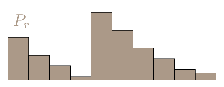
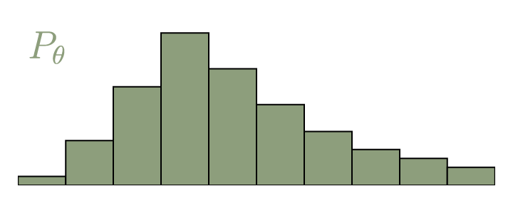
For discrete probability distributions, the Wasserstein distance is also descriptively called the earth mover’s distance (EMD). If we imagine the distributions as different heaps of a certain amount of earth, then the EMD is the minimal total amount of work it takes to transform one heap into the other. Work is defined as the amount of earth in a chunk times the distance it was moved. Let’s call our discrete distributions $P_r$ and $P_\theta$, each with $l$ possible states $x$ or $y$ respectively, and take two arbitrary distributions as an example.
Calculating the EMD is in itself an optimization problem: There are infinitely many ways to move the earth around, and we need to find the optimal one. We call the transport plan that we are trying to find $\gamma(x,y)$. It simply states how we distribute the amount of earth from one place $x$ over the domain of $y$, or vice versa.
To be a valid transport plan, the constraints $\sum_x \gamma(x,y) = P_r(y)$ and $\sum_y \gamma(x,y) = P_\theta(x)$ must of course apply. This ensures that following this plan yields the correct distributions. Equivalently, we can call $\gamma$ a joined probability distribution and require that $\gamma \in \Pi(P_r, P_\theta)$, where $\Pi(P_r, P_\theta)$ is the set of all distributions whose marginals are $P_r$ or $P_\theta$ respectively. To get the EMD, we have to multiply every value of $\gamma$ with the Euclidian distance between $x$ and $y$. With that, the definition of the Earth mover’s distance is:
\[\mathrm{EMD}(P_r, P_\theta) = \inf_{\gamma \in \Pi} \, \sum\limits_{x,y} \Vert x - y \Vert \gamma (x,y) = \inf_{\gamma \in \Pi} \ \mathbb{E}_{(x,y) \sim \gamma} \Vert x - y \Vert\]If you’re not familiar with the expression $\inf$, it stands for infimum, or greatest lower bound. It is simply a slight mathematical variation of the minimum. The opposite is $\sup$ or supremum, roughly meaning maximum, which we will come across later. We can also set $\mathbf{\Gamma} = \gamma(x,y)$ and $\mathbf{D} = \Vert x - y \Vert$, with $\mathbf{\Gamma}, \mathbf{D} \in \mathbb{R}^{l \times l}$. Now we can write
\[\mathrm{EMD}(P_r, P_\theta) = \inf_{\gamma \in \Pi} \, \langle \mathbf{D}, \mathbf{\Gamma} \rangle_\mathrm{F}\]where $\langle , \rangle_\mathrm{F}$ is the Frobenius inner product (sum of all the element-wise products).
Linear Programming
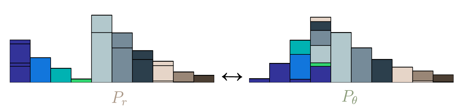
In the picture above you can see the optimal transport plan $\mathbf{\Gamma}$. It can be calculated using the generic method of Linear Programming (LP). With LP, we can solve problems of a certain canonical form: Find a vector $\mathbf{x} \in \mathbb{R}^n$ that minimizes the cost $z = \mathbf{c}^T \mathbf{x}, \ \mathbf{c} \in \mathbb{R}^n$. Additionally, $\mathbf{x}$ is constrained by the equation $\mathbf{A} \mathbf{x} = \mathbf{b}, \ \mathbf{A} \in \mathbb{R}^{m \times n}, \mathbf{b} \in \mathbb{R}^m$ and $\mathbf{x} \geq \mathbf{0}$.
To cast our problem of finding the EMD into this form, we have to flatten $\mathbf{\Gamma}$ and $\mathbf{D}$:
\[\begin{align} \mathbf{x} &= \mathrm{vec}(\mathbf{\Gamma}) \\ \mathbf{c} &= \mathrm{vec}(\mathbf{D}) \\ \end{align}\]This means $n = l^2$. For the constraints, we concatenate the target distributions, which makes $m=2l$:
\[\mathbf{b} = \begin{bmatrix} P_r \\ P_\theta\end{bmatrix}\]For $\mathbf{A}$, we have to construct a large sparse binary matrix that picks out the values from $\mathbf{x}$ and sums them to get $\mathbf{b}$. This schematic should make it clear:
\[\newcommand\FixWidth[1]{ \hspace{2.2em} \llap{#1}} \begin{array}{rc} & \left. \left[ \begin{array} {rrrr|rrrr} \FixWidth{P_r(x_1)} & \FixWidth{P_r(x_2)} & \FixWidth{\dots} & \FixWidth{P_r(x_n)} & \FixWidth{P_\theta(y_1)} & \FixWidth{P_\theta(y_2)} & \FixWidth{\dots} & \FixWidth{P_\theta(y_n)} \end{array} \right] \, \right\} \; \mathbf{b}^T \\ \\ \mathbf{x} \left\{ \begin{bmatrix} \gamma(x_1, y_1) \\ \gamma(x_1, y_2) \\ \vdots \\ \hline \gamma(x_2, y_1) \\ \gamma(x_2, y_2) \\ \vdots \\ \hline \vdots \\ \hline \gamma(x_n, y_1) \\ \gamma(x_n, y_2) \\ \vdots \\ \end{bmatrix} \right. & \left. \left[ \begin{array}{rrrr|rrrr} 1 & 0 & \dots & 0 & 1 & 0 & \dots & 0 \cr 1 & 0 & \dots & 0 & 0 & 1 & \dots & 0 \cr \vdots & \vdots & \dots & \vdots & \vdots & \vdots & \ddots & \vdots \cr \hline 0 & 1 & \dots & 0 & 1 & 0 & \dots & 0 \cr 0 & 1 & \dots & 0 & 0 & 1 & \dots & 0 \cr \vdots & \vdots & \dots & \vdots & \vdots & \vdots & \ddots & \vdots \cr \hline \FixWidth{\vdots} & \FixWidth{\vdots} & \FixWidth{\vdots} & \FixWidth{\vdots} & \FixWidth{\vdots} & \FixWidth{\vdots} & \FixWidth{\vdots} & \FixWidth{\vdots} \cr \hline 0 & 0 & \dots & 1 & 1 & 0 & \dots & 0 \cr 0 & 0 & \dots & 1 & 0 & 1 & \dots & 0 \cr \vdots & \vdots & \dots & \vdots & \vdots & \vdots & \ddots & \vdots \cr \end{array} \right] \right\} \mathbf{A}^T \end{array}\]With that, we can call a standard LP routine, for example linprog() from scipy.
import numpy as np
from scipy.optimize import linprog

# We construct our A matrix by creating two 3-way tensors,
# and then reshaping and concatenating them
A_r = np.zeros((l, l, l))
A_t = np.zeros((l, l, l))

for i in range(l):
	for j in range(l):
		A_r[i, i, j] = 1
		A_t[i, j, i] = 1

A = np.concatenate((A_r.reshape((l, l**2)), A_t.reshape((l, l**2))), axis=0)
b = np.concatenate((P_r, P_t), axis=0)
c = D.reshape((l**2))

opt_res = linprog(c, A_eq=A, b_eq=b)
emd = opt_res.fun
gamma = opt_res.x.reshape((l, l))
Now we have our transference plan, as well as the EMD.
Dual Form
Unfortunately, this kind of optimization is not practical in many cases, certainly not in domains where GANs are usually used. In our example, we use a one-dimensional random variable with ten possible states. The number of possible discrete states scales exponentially with the number of dimensions of the input variable. For many applications, e.g. images, the input can easily have thousands of dimensions. Even an approximation of $\gamma$ is then virtually impossible.
But actually we don’t care about $\gamma$. We only want a single number, the EMD. Also, we want to use it to train our generator network, which generates the distribution $P_\theta$. To do this, we must be able to calculate the gradient $\nabla_{P_\theta} \mathrm{EMD}(P_r, P_\theta)$. Since $P_r$ and $P_\theta$ are only constraints of our optimization, this not possible in any straightforward way.
As it turns out, there is another way of calculating the EMD that is much more convenient. Any LP has two ways in which the problem can be formulated: The primal form, which we just used, and the dual form.
\[\begin{array}{c|c} \mathbf{primal \ form:} & \mathbf{dual \ form:}\\ \begin{array}{rrcl} \mathrm{minimize} \ & z & = & \ \mathbf{c}^T \mathbf{x}, \\ \mathrm{so \ that} \ & \mathbf{A} \mathbf{x} & = & \ \mathbf{b} \\ \mathrm{and}\ & \mathbf{x} & \geq &\ \mathbf{0} \end{array} & \begin{array}{rrcl} \mathrm{maximize} \ & \tilde{z} & = & \ \mathbf{b}^T \mathbf{y}, \\ \mathrm{so \ that} \ & \mathbf{A}^T \mathbf{y} & \leq & \ \mathbf{c} \\ \\ \end{array} \end{array}\]By changing the relations between the same values, we can turn our minimization problem into a maximization problem. Here the objective $\tilde{z}$ directly depends on $\mathbf{b}$, which contains the our distributions $P_r$ and $P_\theta$. This is exactly that we want. It is easy to see that $\tilde{z}$ is a lower bound of $z$:
\[z = \mathbf{c}^T \mathbf{x} \geq \mathbf{y}^T \mathbf{A} \mathbf{x} = \mathbf{y}^T \mathbf{b} = \tilde{z}\]This is called the Weak Duality theorem. As you might have guessed, there also exists a Strong Duality theorem, which states that, should we find an optimal solution for $\tilde{z}$, then $z=\tilde{z}$. Proving it is a bit more complicated and requires Farkas theorem as an intermediate result.
Farkas Theorem
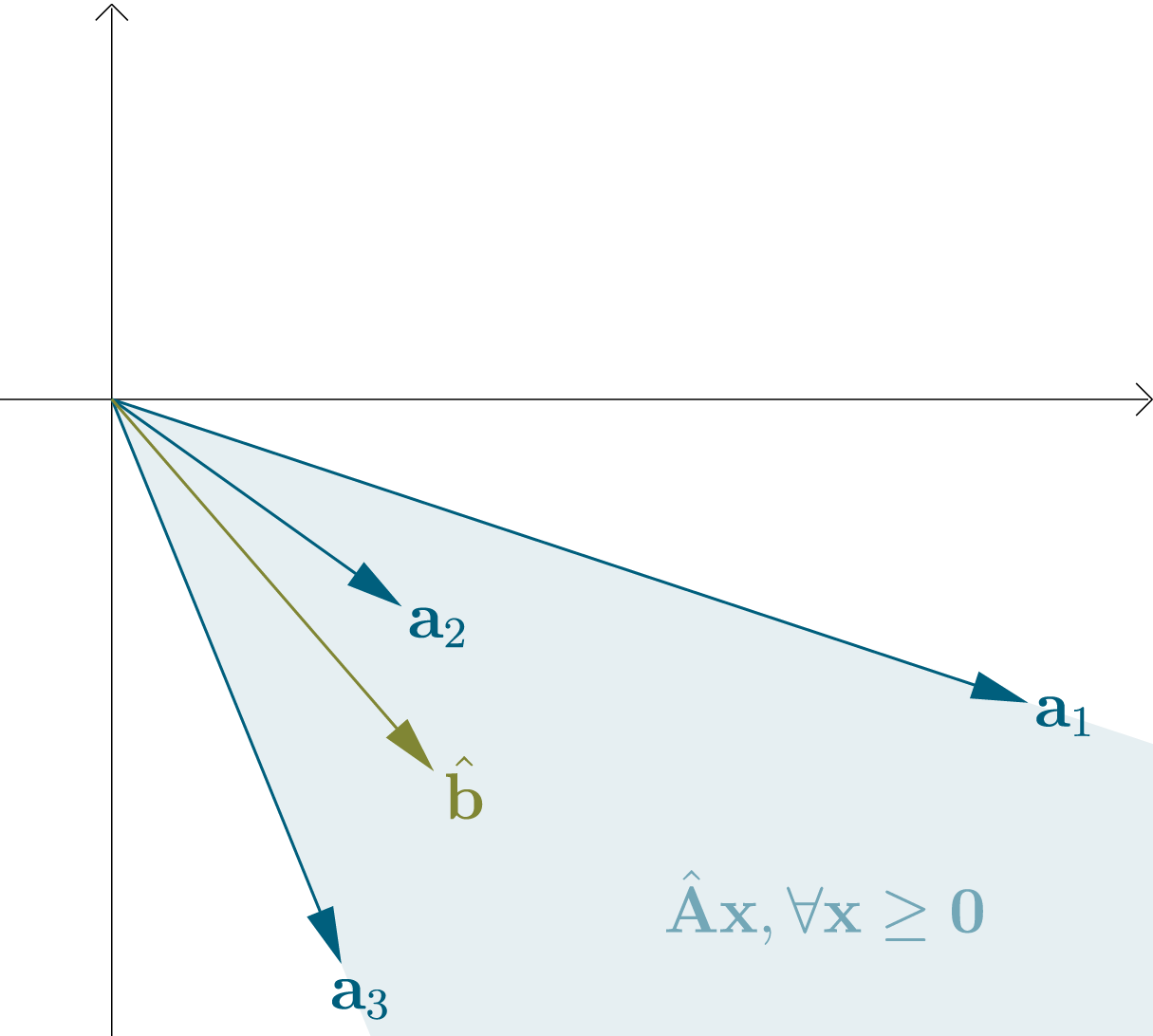
We can regard the columns of a matrix $\hat{\mathbf{A}} \in \mathbb{R}^{d \times n}$ as vectors $\mathbf{a}_{1}, \mathbf{a}_{2}, …, \mathbf{a}_{n}\in \mathbb{R}^{d}$. The set of all possible linear combinations of these vectors with nonnegative coefficients is a convex cone with its apex (peak) at the origin (note that a convex cone could also potentially cover the whole $\mathbb{R}^{d}$ space). We can combine these coefficients in a vector $\mathbf{x} \in \mathbb{R}^{n}_{\geq 0}$.
For a vector $\hat{\mathbf{b}} \in \mathbb{R}^{d}$, there are now exactly two possibilities: Either $\hat{\mathbf{b}}$ is contained in the cone, or not. If $\hat{\mathbf{b}}$ is not contained, then we can fit a hyperplane $h$ that goes through the origin between the convex cone and $\hat{\mathbf{b}}$. We can define it in terms of only its normal vector $\hat{\mathbf{y}} \in \mathbb{R}^{d}$. If a vector $\mathbf{v} \in \mathbb{R}^{d}$ lies on $h$, then $\mathbf{v}^T \hat{\mathbf{y}} = 0$, if $\mathbf{v}$ lies in the upper half-space of $h$ (the same side as $\hat{\mathbf{y}}$), then $\mathbf{v}^T \hat{\mathbf{y}} > 0$ and if $\mathbf{v}$ lies in the lower half-space (the opposite side of $\hat{\mathbf{y}}$), then $\mathbf{v}^T \hat{\mathbf{y}} < 0$. As we specified, if $h$ exists, then $\hat{\mathbf{b}}$ lies in a different half-space than all vectors $\mathbf{a}_i$.
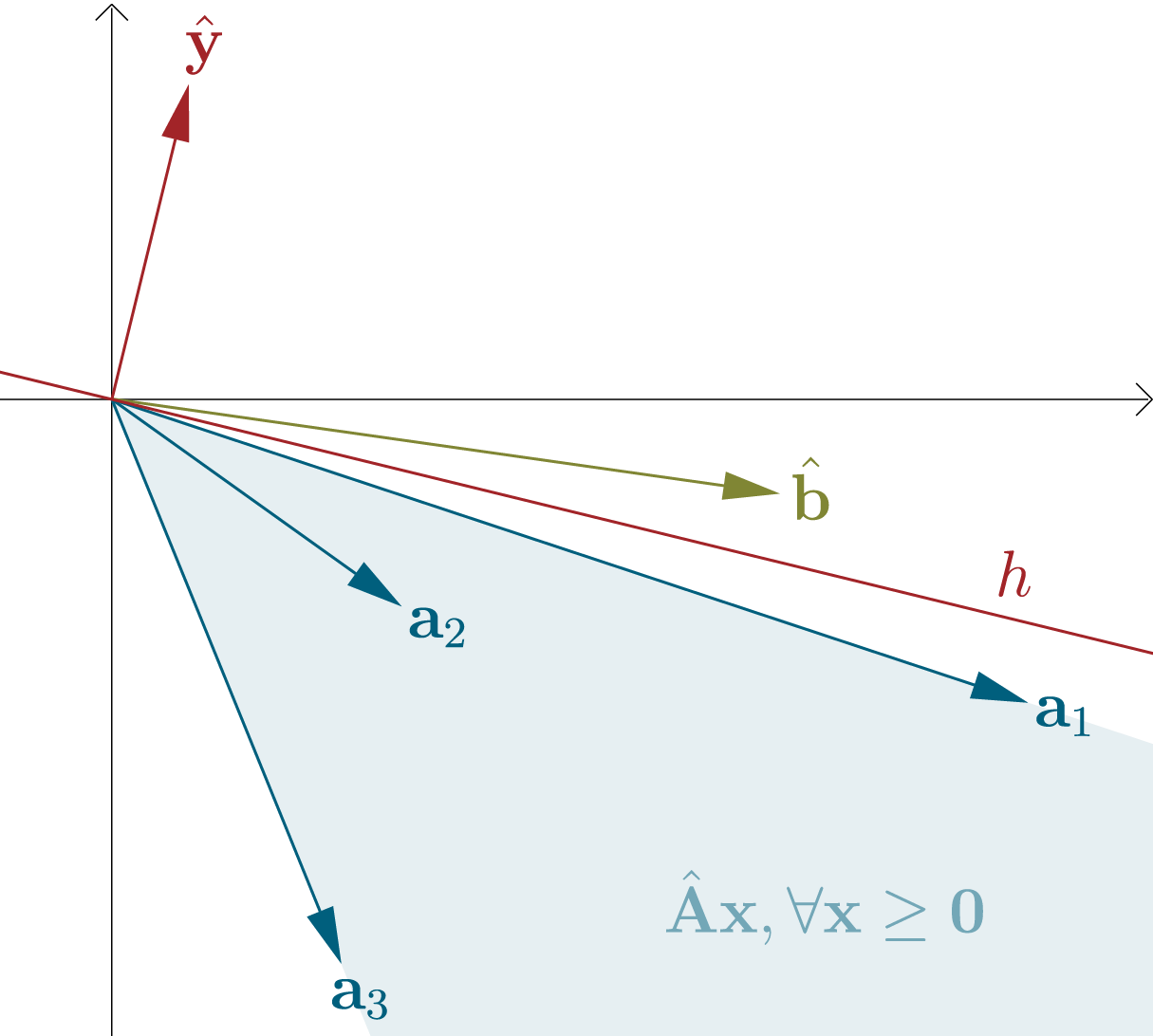
Summarized, exactly one of the following statements is true:
- $(1)$ There exists $\mathbf{x} \in \mathbb{R}^{n}$, so that $\hat{\mathbf{A}} \mathbf{x} = \hat{\mathbf{b}}$ and $\mathbf{x} \geq \mathbf{0}$
- $(2)$ There exists $\hat{\mathbf{y}} \in \mathbb{R}^{d}$, so that $\hat{\mathbf{A}}^T \hat{\mathbf{y}} \leq \mathbf{0}$ and $\hat{\mathbf{b}}^T \hat{\mathbf{y}} > 0$
This is called Farkas theorem, or Farkas alternatives. There exist slightly different versions and several proofs, but what we showed is sufficient for our purposes.
Strong Duality
The trick for the second part of this proof is to construct a problem that is related to our original LP forms, but with one additional dimension and in such a way that $\hat{\mathbf{b}}$ lies right at the edge of the convex cone. Then according to Farkas, for some $\hat{\mathbf{y}}$, the corresponding hyperplane comes arbitrarily close to $\hat{\mathbf{b}}$. From this, in combination with the Weak Duality theorem, we will proof the Strong Duality.
Let the minimal solution to the primal problem be ${z^* } = \mathbf{c}^T \mathbf{x}^{* }$. Then we define
\[\hat{\mathbf{A}} = \begin{bmatrix} \mathbf{A} \\ -\mathbf{c}^T \end{bmatrix}, \ \ \ \hat{\mathbf{b}}_\epsilon = \begin{bmatrix} \mathbf{b} \\ -z^* + \epsilon \end{bmatrix}, \ \ \ \hat{\mathbf{y}} = \begin{bmatrix} \mathbf{y} \\ \alpha \end{bmatrix}\]with $\epsilon, \alpha \in \mathbb{R}$. For $\epsilon = 0$, we have Farkas case $(1)$, because $\hat{\mathbf{A}} \mathbf{x}^* = \hat{\mathbf{b}}_0$. For $\epsilon > 0$, there exists no nonnegative solution (because $z^{* }$ is already minimal) and we have Farkas case $(2)$. This means there exist $\mathbf{y}$ and $\alpha$, such that
\[\begin{bmatrix} \mathbf{A} \\ -\mathbf{c}^T \end{bmatrix}^T \begin{bmatrix} \mathbf{y} \\ \alpha \end{bmatrix} \leq \mathbf{0}, \ \ \ \ \begin{bmatrix} \mathbf{b} \\ -z^* + \epsilon \end{bmatrix} \begin{bmatrix} \mathbf{y} \\ \alpha \end{bmatrix} > 0\]or equivalently
\[\mathbf{A}^T \mathbf{y} \leq \alpha \mathbf{c}, \ \ \mathbf{b}^T \mathbf{y} > \alpha(z^* - \epsilon).\]The way we constructed it, we can find $\hat{\mathbf{y}}$ so that additionally $\hat{\mathbf{b}}_0 \hat{\mathbf{y}} = 0$. Then changing $\epsilon$ to any number greater than $0$ has to result in $\hat{\mathbf{b}}_0 \hat{\mathbf{y}} > 0$. In our specific problem, this is only possible if $\alpha > 0$, because $z^* > 0$. We showed that $\hat{\mathbf{y}}$ is simply the normal vector of a hyperplane, and because of that we can freely scale it to any magnitude greater than zero. Particularly, we can scale it so that $\alpha = 1$. This means there exists a vector $\mathbf{y}$, so that
\[\mathbf{A}^T \mathbf{y} \leq \mathbf{c}, \ \ \mathbf{b}^T \mathbf{y} > z^* - \epsilon.\]We see that $\tilde{z} := z^* - \epsilon$ for any $\epsilon > 0$ is a feasible value of the objective of our dual problem. From the Weak Duality theorem, we know that $\tilde{z} \leq z^{* }$. We just showed that $\tilde{z}$ can get arbitrarily close to $z^{* }$. This means the optimal (maximal) value of our dual form is also $z^{* }$.
Dual Implementation
Now we can confidently use the dual form to calculate the EMD. As we showed, the maximal value $\tilde{z}^* = \mathbf{b}^T \mathbf{y}^{* }$ is the EMD. Let’s define
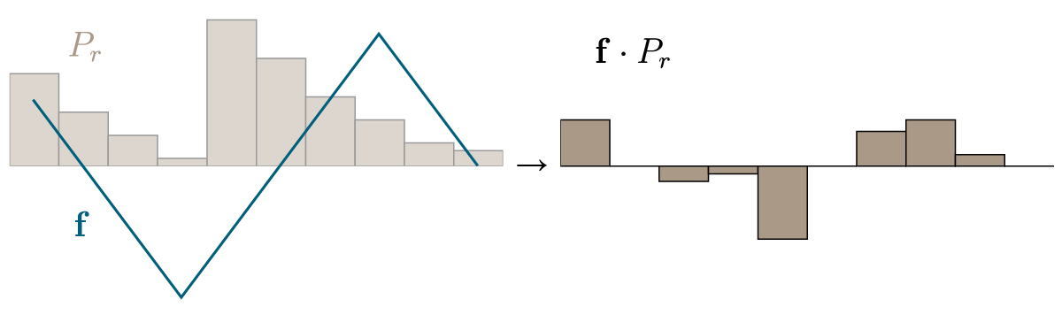
\[\mathbf{y}^* = \begin{bmatrix} \mathbf{f} \\ \mathbf{g} \end{bmatrix}\]with $\mathbf{f}, \mathbf{g} \in \mathbb{R}^d$. This means $\mathrm{EMD}(P_r, P_\theta) = \mathbf{f}^T P_r + \mathbf{g}^T P_\theta$. Recall the constraints of the dual form: $\mathbf{A}^T \mathbf{y} \leq \mathbf{c}$.
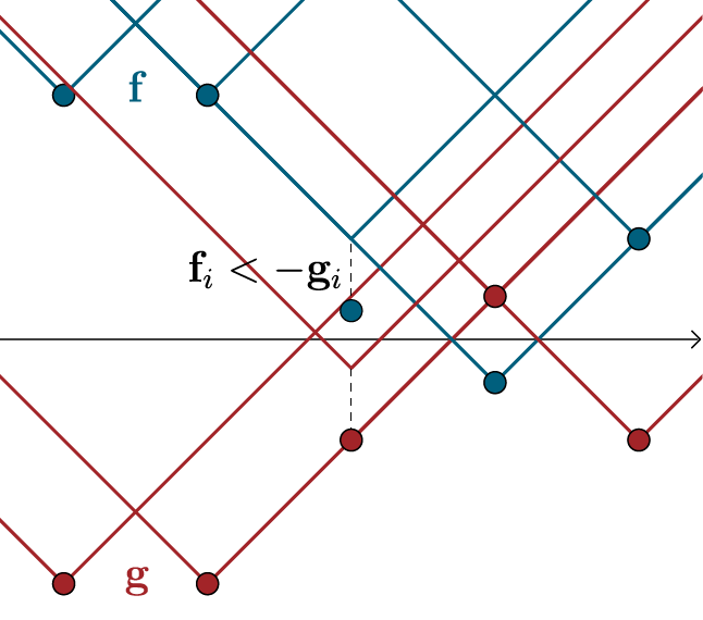
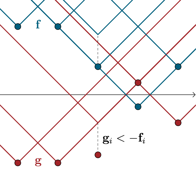
\[\newcommand\FixWidth[1]{ \hspace{1.6em} \llap{#1}} \begin{array}{rc} & \left. \left[ \begin{array} {rrr|rrr|r|rrr} \FixWidth{\mathbf{D}_{1,1}} & \FixWidth{\mathbf{D}_{1,2}} & \FixWidth{\dots} & \FixWidth{\mathbf{D}_{2,1}} & \FixWidth{\mathbf{D}_{2,2}} & \FixWidth{\dots} & \FixWidth{\dots} & \FixWidth{\mathbf{D}_{n,1}} & \FixWidth{\mathbf{D}_{ n,2}} & \FixWidth{\dots} \end{array} \right] \, \right\} \; \mathbf{c}^T \\ \\ \mathbf{y} \left\{ \begin{bmatrix} f(x_1) \\ f(x_2) \\ \vdots \\ f(x_n) \\ \hline g(x_1) \\ g(x_2) \\ \vdots \\ g(x_n) \\ \end{bmatrix} \right. & \left. \;\; \left[ \begin{array} {rrr|rrr|r|rrr} 1 & 1 & \dots & 0 & 0 & \dots & \dots & 0 & 0 & \dots \cr 0 & 0 & \dots & 1 & 1 & \dots & \dots & 0 & 0 & \dots \cr \vdots & \vdots & \vdots & \vdots & \vdots & \vdots & \dots & \vdots & \vdots & \vdots \cr 0 & 0 & \dots & 0 & 0 & \dots & \dots & 1 & 1 & \dots \cr \hline 1 & 0 & \dots & 1 & 0 & \dots & \dots & 1 & 0 & \dots \cr 0 & 1 & \dots & 0 & 1 & \dots & \dots & 0 & 1 & \dots \cr \vdots & \vdots & \ddots & \vdots & \vdots & \ddots & \dots & \vdots & \vdots & \ddots \cr \FixWidth{0} & \FixWidth{0} & \FixWidth{\dots} & \FixWidth{0} & \FixWidth{0} & \FixWidth{\dots} & \FixWidth{\dots} & \FixWidth{0} & \FixWidth{0} & \FixWidth{\dots} \end{array} \right] \right\} \mathbf{A}\phantom{^T ;} \end{array}\]We have written the vectors $\mathbf{f}$ and $\mathbf{g}$ as values of the functions $f$ and $g$. The constraints can be summarized as $f(x_i) + g(x_j) \leq \mathbf{D}_{i,j}$. The case $i=j$ yields $g(x_i) \leq -f(x_i)$ for all $i$, because $\mathbf{D}_{i,i} = 0$. Since $P_r$ and $P_\theta$ are nonnegative, to maximize our objective, $\sum_i \mathbf{f}_i + \mathbf{g}_i$ has to be as great as possible. This sum has a maximum value of $0$, which we achieve with $g = - f$. This remains true given all additional constraints: Choosing $g(x_{i}) < - f(x_{i})$ would only make sense if it had benefits for values $f(x_{j})$ and $g(x_{j})$ with $j \neq i$. Since $f(x_{j})$ and $g(x_{j})$ remain upper-bounded by the other constraints, this is not the case.
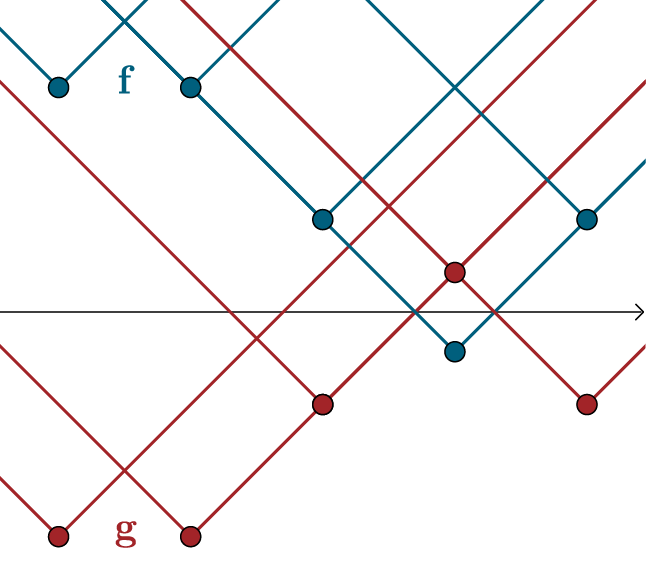
For $g = - f$ the constraints become $f(x_i) - f(x_j) \leq \mathbf{D}_{i,j}$ and $f(x_i) - f(x_j) \geq -\mathbf{D}_{i,j}$. If we see the values $f(x_i)$ as connected with line segments, this means that the upward and the downward slope of these segments is limited. In our case, where we use Euclidian distances, these slope limits are $1$ and $-1$. We call this constraint Lipschitz continuity (with Lipschitz constant $1$) and write $\lVert f \lVert_{L \leq 1}$. With that, our dual form of the EMD is
\[\mathrm{EMD}(P_r, P_\theta) = \sup_{\lVert f \lVert_{L \leq 1}} \ \mathbb{E}_{x \sim P_r} f(x) - \mathbb{E}_{x \sim P_\theta} f(x).\]The implementation is straightforward:
# linprog() can only minimize the cost, because of that
# we optimize the negative of the objective. Also, we are
# not constrained to nonnegative values.
opt_res = linprog(-b, A, c, bounds=(None, None))

emd = -opt_res.fun
f = opt_res.x[0:l]
g = opt_res.x[l:]
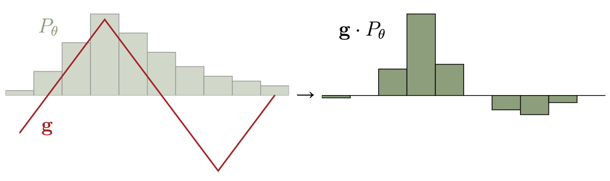
As we see, the optimal strategy is of course to set $f(x)$ to high values where $P_r(x) > P_\theta(x)$, and to low values where $P_\theta > P_r$.
Wasserstein Distance
Lastly, we have to consider continuous probability distributions. We can of course view them intuitively as discrete distributions with infinitely many states and use a similar reasoning as described so far. But as I mentioned at the beginning, we will try something neater. Let our continuous distributions be $p_r$ and $p_\theta$, and the set of joined distributions with marginals $p_r$ and $p_\theta$ be $\pi(p_r, p_\theta)$. Then the Wasserstein distance is defined as
\[W(p_r, p_\theta) = \inf_{\gamma \in \pi} \iint\limits_{x,y} \lVert x - y \lVert \gamma (x,y) \, \mathrm{d} x \, \mathrm{d} y = \inf_{\gamma \in \pi} \mathbb{E}_{x,y \sim \gamma} \left[ \lVert x - y \lVert \right].\]If we add suitable terms, we can remove all constraints on the distribution $\gamma$. This is done by adding an additional optimization over a function $f: x \mapsto k \in \mathbb{R}$, which rules out all $\gamma \notin \pi$ as solutions:
\[\begin{array}{rl} W(p_r, p_\theta) & = \inf\limits_{\gamma \in \pi} \mathbb{E}_{x,y \sim \gamma} [ \lVert x - y \lVert ] \\ &\begin{array}{cc} = \inf\limits_{\gamma } \mathbb{E}_{x,y \sim \gamma} [ \lVert x - y \lVert & + \; \underbrace{\sup\limits_{f} \mathbb{E}_{s \sim p_r}[f(s)] - \mathbb{E}_{t \sim p_\theta}[f(t)] - \left( f(x) - f(y) \right)} ] \\ &= \cases{\begin{align} 0, & \ \ \ \mathrm{if \ \gamma \in \mathrm{\pi}} \\ + \infty & \ \ \ \mathrm{else} \end{align}} \end{array}\\ & = \inf\limits_{\gamma} \ \sup\limits_{f} \ \mathbb{E}_{x,y \sim \gamma} [ \lVert x - y \lVert + \mathbb{E}_{s \sim p_r}[f(s)] - \mathbb{E}_{t \sim p_\theta}[f(t)] - \left( f(x) - f(y) \right) ] \end{array}\]Now we have bilevel optimization. This means we take the optimal solution of the inner optimization ($\sup_f$) for every value of the outer optimization ($\inf_\gamma$), and from these possible solutions choose the one that is optimal for the outer optimization. To continue, we have to make use of the minimax-principle, which says that in certain cases we can invert the order of $\inf$ and $\sup$ without changing the solution. But first we have to show that our problem is indeed such a case.
Consider some function $g: A, B \rightarrow \mathbb{R}$. Let $g(\hat{a}, \hat{b}) = \inf_{a \in A} \sup_{\ b \in B} g(a,b)$ (‘the least of all maxima’) and $g(\hat{a}’, \hat{b}’) = \sup_{\ b \in B} \inf_{a \in A} g(a,b)$ (‘the greatest of all minima’). The argument that $g(\hat{a}, \hat{b}) \geq g(\hat{a}’, \hat{b}’)$ is simple: Any $g(\hat{a}, \hat{b})$ is automatically allowed as a candidate for the infimum of $\sup_{\ b \in B} \inf_{a \in A} g(a,b)$, but not the other way around. This is equivalent to the statement $\sup_b g(a’, b) \geq g(a’, b’) \geq \inf_a g(a, b’) \forall a’, b’$, which is true by definition.
For $g(\hat{a}, \hat{b}) > g(\hat{a}’, \hat{b}’)$, at least one of these statements must be true:
- $g(\hat{a}+t, \hat{b}) < g(\hat{a}, \hat{b})$ for some $t \neq 0$. This is only possible if $\sup_{\ b \in B} g(a,b)$ is not convex in $a$, because $g(\hat{a}, \hat{b})$ is already an infimum for $\hat{a}$.
- $g(\hat{a}’, \hat{b}’+t) > g(\hat{a}’, \hat{b}’)$ for some $t \neq 0$. This is only possible if $\inf_{\ a \in A} g(a,b)$ is not concave in $b$, because $g(\hat{a}’, \hat{b}’)$ is already a supremum for $\hat{b}’$.
This means of course that, if $\sup_{\ b \in B} g(a,b)$ is convex and $\inf_{\ a \in A} g(a,b)$ is concave, then the minimax principle applies and $g(\hat{a}, \hat{b}) = g(\hat{a}’, \hat{b}’)$. In our case, we can above already see from the underbrace that the convexity condition is met. Let’s try changing to $\sup \inf$:
\[\begin{array}{ll} &\phantom{= , } \sup\limits_{f} \ \inf\limits_{\gamma} \ \mathbb{E}_{x,y \sim \gamma} [ \lVert x - y \lVert + \mathbb{E}_{s \sim p_r}[f(s)] - \mathbb{E}_{t \sim p_\theta}[f(t)] - (f(x) - f(y)) ] \\ &\begin{array}{cc} = \sup\limits_{f} \ \mathbb{E}_{s \sim p_r}[f(s)] - \mathbb{E}_{t \sim p_\theta}[f(t)] + & \underbrace{ \inf\limits_{\gamma} \ \mathbb{E}_{x,y \sim \gamma} [ \lVert x - y \lVert - ( f(x) - f(y))} ] \\ &= \cases{\begin{align} 0, & \ \ \ \mathrm{if} \ \| f \| {}_{L} \leq 1\\ - \infty & \ \ \ \mathrm{else} \end{align}} \end{array} \end{array}\]We see that the infimum is concave, as required. Because all functions $f$ that are Lipschitz continuous produce the same optimal solution for $\inf_\gamma$, and only they are feasible solutions of $\sup_f$, we can turn this condition into a constraint. With that, we have the dual form of the Wasserstein distance:
\[\begin{align} W(p_r, p_\theta) & = \sup_{f} \ \mathbb{E}_{s \sim p_r}[f(s)] - \mathbb{E}_{t \sim p_\theta}[f(t)] + \inf_{\gamma} \ \mathbb{E}_{x,y \sim \gamma} [ \lVert x - y \lVert - ( f(x) - f(y)) ] \\ & = \sup_{\lVert f \lVert_{L \leq 1}} \ \mathbb{E}_{s \sim p_r}[f(s)] - \mathbb{E}_{t \sim p_\theta}[f(t)] \end{align}\]This is our case of the Kantorovich-Rubinstein duality. It actually holds for other metrics than just the Euclidian metric we used. But the function $f$ is suitable to be approximated by a neural network, and this version has the advantage that the Lipschitz continuity can simply be achieved by clamping the weights.
Leave a Comment