Immersions - Visualizing and sonifying how an artificial ear hears music
Visualizing and sonifying how an artificial ear hears music
\[\def\sb{_}\]This project lets us interact with and explore an audio processing neural network, or what I call an “artificial ear”. This network was trained in an unsupervised way on various music datasets using a contrastive predictive coding method. There are two modes of showing its inner workings - one is visual, the other is sonic. For the visualization, first, the neurons of the network are laid out in two-dimensional space, then their activation is shown at every moment, depending on the input, in real-time. To make audible how music sound to the artificial ear, an optimization procedure generates sounds that specifically activate certain neurons in the network. In case you’re interested, please see the the paper or the poster, as well as the visualization code (that you could use to visualize your own networks)!
If you want to skip the theory, you can jump straight down to the audio and video demonstrations starting in the visualization section.
Introduction
Although neural networks are often described as black boxes, there exist methods to make us see and hear what is going on inside a neural network. A well-known example of this is the DeepDream technique that generates bizarre psychedelic but strangely familiar pictures. A related approach can be used to make audible the innards of sound processing neural nets. The first thing we need is a model we want to examine. It is trained on musical data using a self-supervised training algorithm. Then the basic idea is the following: The starting point is an arbitrary sound clip (e.g. silence, noise, or a drum loop). This clip will be modified by the optimization procedure in a way that stimulates a certain region in the neural net. The changed clip can then be used as a basis for a new optimization. This way you obtain sounds that are generated by the neural network in a freely associative way. One of the most important properties of neural networks is that they process information on different levels of abstraction. An activation in some region of the net thus may, for example, be associated with short and simple sounds or noises, a different region with a more complex musical phenomenon, such as rhythm, phrase or key. For what exactly a neural networks listens depends on the data it was trained on, as well as on the task it is specialized to accomplish. This means to different nets music will sound differently. All this can be directly experienced with the Immersions project. For this, I developed a setup that allows - not unlike a DJ mixing console - the generation, visualization and control of sound in real-time. The contributions presented here are the following:
- The application and evaluation of Contrastive Predictive Coding for self-supervised representation learning on spectral representations of music. For this, new fully convolutional architectures for both encoder and autoregressive model are used and evaluated.
- A method of finding a clear visual representation of a neural network using the multilevel force graph layout technique and visualizing activations of all neurons in real-time.
- Transfer of the principles of feature visualization to the sound domain, allowing the sonification of features a model relies on.
- Development of a system that allows the real-time control and exploration of the sonic feature space.
Contrastive Predictive Coding
In the centre of this project stands an “artificial ear”, meaning a sound processing neural network. It has been shown that analogies exist between convolutional neural networks (ConvNets) and the human auditory cortex (see, for example, this paper). Of course, the human auditory system is not a classification network, we usually don’t learn with the help of explicit labels. The question of the actual learning mechanisms in the brain is highly contested, but a promising candidate, especially for perceptual learning, might be predictive coding. Here future neural responses to stimuli are predicted and then compared to the actually occurred responses. The learning entails reducing the discrepancy between prediction and reality.
One method of using the idea of predictive coding for self-supervised learning in artificial neural networks is presented in Representation Learning with Contrastive Predictive Coding. For this so-called contrastive predictive coding you need two models:
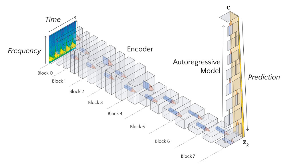
The encoder model builds a compressed encoding $\mathbf{z}\sb{t}$ of the signal for each time step $t$ and the autoregressive model summarizes multiple sequential encodings into a vector $\mathbf{c}$. The encoding $k$ time steps in the future, $\mathbf{z}_{k}$, is predicted by a different learnt linear transformation $\mathbf{M}_k$ of $\mathbf{c}$ for each time step. The time steps $k$ are counted from the latest point $t$ for which the autoregressive model had access to the encoding $\mathbf{z}_t$. The loss for each mini-batch is calculated as follows:
\[\mathcal{L}_{CPC} = - \sum_{n, k} \log \frac{\exp(\mathbf{z}^T_{n, k} \mathbf{M}_k \mathbf{c}_n)} {\sum_m \exp(\mathbf{z}^T_{m, k} \mathbf{M}_k \mathbf{c}_n)}\]Both $n$ and $m$ are indices of the mini-batch dimension. The numerator is a scalar score that measures how well the prediction matches the correct encoding. It is divided by the sum of the scores that measure the prediction against all encodings of the current mini-batch. Minimizing $\mathcal{L}\sb{CPC}$ maximizes the mutual information between $\mathbf{c}$ and future encodings $\mathbf{z}_{k}$. This means that there is little incentive to encode high-frequency noise since this information is not shared over longer time scales. Instead, the model can learn to focus on “slow” features that are useful for differentiating those signals.
Using contrastive predictive coding frees us to choose out training data without many constraints. No expensively labelled datasets are required, the model learns to make sense of any inputs it is given.
Model Architecture
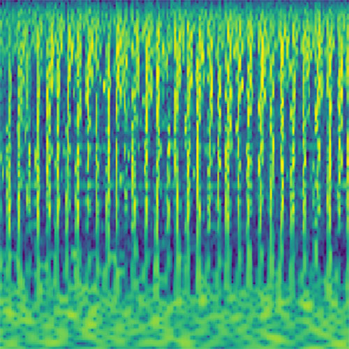
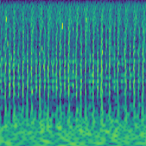
The encoder network receives as input a scaleogram representation of an audio clip. A scaleogram is the result of a constant-Q or a wavelet transformation of the audio signal and comes quite close to the representation that the cochlea passes on to the brain. For the purpose of input optimization, which will be described below, the transformation from a raw audio signal to the scaleogram has to be differentiable. Fortunately, it can simply be implemented as a 1D convolutional layer with fixed weights in any standard deep learning framework. For each frequency band, two channels of the kernels are assigned to represent the real and imaginary part of the corresponding finite impulse response filter. The stride parameter is equivalent to the hop length of the transformation. The output of this layer can be reshaped to have the dimensions time, frequency, and real/imaginary. This representation is then converted into polar coordinates. The amplitude is squared and logarithmically scaled. This results in the two-dimensional scaleogram representation, which is the input to the encoder network. Additionally, the phase part is used as the second channel for the input, although I did not find that this improves the performance noticeably.
As encoder serves a 2D-ConvNet, similar to the kind common in computer vision and image processing. It is based on the ResNet architecture, with a few modifications: Since the model is trained on a prediction task, we use only causal convolutions. In practice, this simply means padding only at the start of the time dimension for both convolution and pooling layers. Also, in addition to the usual quadratic kernels, we apply kernels that only span the frequency dimension and are supposed to detect overtones and harmonies.
The output of the encoder, only the dimensions time and channel are left. They represent timestep and features of $\mathbf{z}_{k}$. In the original paper, a recurrent neural network is used as the autoregressive model. We use a causal 1D-ConvNet instead, similarly to the encoder network employing ReLU nonlinearities, residual connections, max pooling and batch normalization.
| Block | Channels | Conv 1 | Conv 2 |
|---|---|---|---|
| 0 | 8 | 3x3 pool2 | 1x25 |
| 1 | 16 | 1x3 | 1x3 |
| 2 | 32 | 3x3 | 1x15 |
| 3 | 64 | 1x3 | 1x3 |
| 4 | 128 | 3x3 pool 2 | 1x15 |
| 5 | 256 | 1x3 | 1x3 |
| 6 | 512 | 3x3 | 1x5 |
| 7 | 512 | 1x3 | 1x3 |
| Block | Channels | Conv 1 |
|---|---|---|
| 0 | 512 | 4 |
| 1 | 512 | 4 |
| 2 | 512 | 1 pool 2 |
| 3 | 512 | 4 |
| 4 | 256 | 4 |
| 5 | 256 | 1 pool 2 |
| 6 | 256 | 4 |
| 7 | 256 | 1 |
| 8 | 256 | 4 |
Experiment
For the experiments, the inputs are audio clips with a length of four seconds at a sample rate of 44.1 kHz. The scaleogram has the hop length 1024 and 216 frequency bins (starting at 40 Hz, 24 bins per octave), resulting in the input size 172 x 216. The encoder model has two pooling layers with stride 2, which leads the time steps of the encodings $\mathbf{z}\sb{t}$ to have a length of ca. 93 ms. The autoregressive model integrates 42 consecutive encodings into one representation $\mathbf{c}$. From $\mathbf{c}$, 16 future encodings $\mathbf{z}_{k}$ are predicted, skipping the first 4 immediate next time steps.
I trained the same model on two different datasets: one consisting of about 40 hours of house music mixes, and the other one of 200 hours of classical piano music. To evaluate the performance of the CPC training, the learned representations were used in a test tasks classification setting. For this, the audio data of the test tasks were fed into the trained models and the resulting features $\mathbf{c}$ were saved. Those features were provided with the relevant labels and split into a training and an evaluation set. A linear classifier was fitted with the training set.
The first task was to assign audio clips to the house track it was extracted from (with a total of 15 possible tracks). For the second task the composer of given the audio had to be classified (the samples were also taken from the MAESTRO dataset). As a baseline, the whole architecture was trained directly in a supervised setting from scratch for both of the tasks.
I also trained the models additionally with a slight modification of the CPC algorithm: Instead of contrasting the prediction scores with the other samples from the mini-batch, they are also contrasted with different time steps (score across time steps, SAT):
\[\mathcal{L}_{CPC \, SAT} = - \sum_{n, k} \log \frac{\exp(\mathbf{z}^T_{n, k} \mathbf{M}_k \mathbf{c}_n)} {\sum_{m, l} \exp(\mathbf{z}^T_{m, l} \mathbf{M}_l \mathbf{c}_n)}\]| Model | house loss | house accuracy | maestro loss | maestro accuracy |
|---|---|---|---|---|
| CPC house | 0.3914 | 90.44 % | 2.212 | 25.36 % |
| CPC house SAT | 0.3583 | 91.81 % | 2.087 | 30.06 % |
| CPC maestro | 0.5131 | 86.83 % | 0.659 | 77.49 % |
| CPC maestro SAT | 0.8789 | 76.62 % | 0.700 | 75.90 % |
| supervised house | 1.563 | 48.25 % | ||
| supervised maestro | 2.744 | 19.70 % |
The performance of the CPC trained models on the test tasks is encouraging, especially when compared to the supervised models. Maybe not surprisingly, the latter show poor performance as there was not enough training data to learn meaningful features for the tasks. The use of SAT loss improves performance only for the model trained on the house dataset. One possible explanation might be that SAT training makes better use of limited data, but can be harmful if enough data is available. It could also depend on the specific nature of the data. For this, further investigation is needed.
Below, for all visualizations and sonifications the CPC maestro model is used.
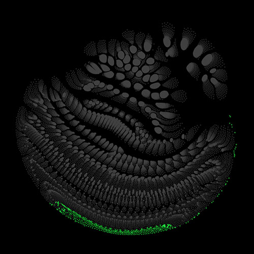
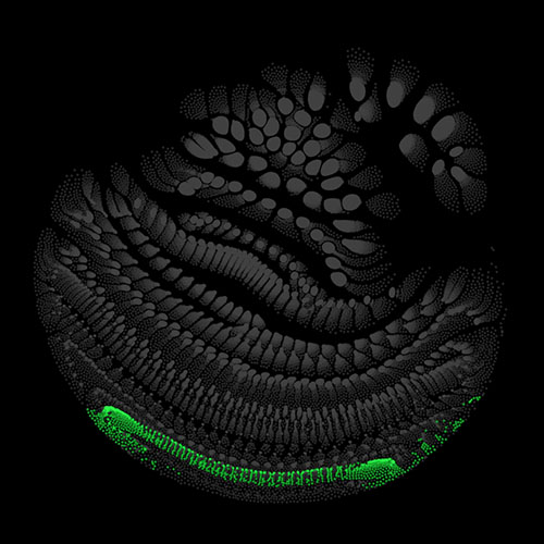
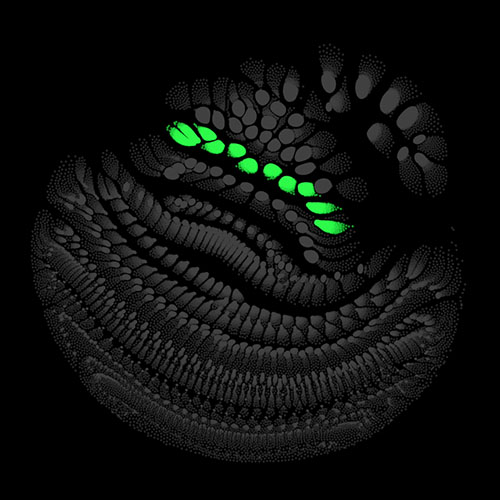
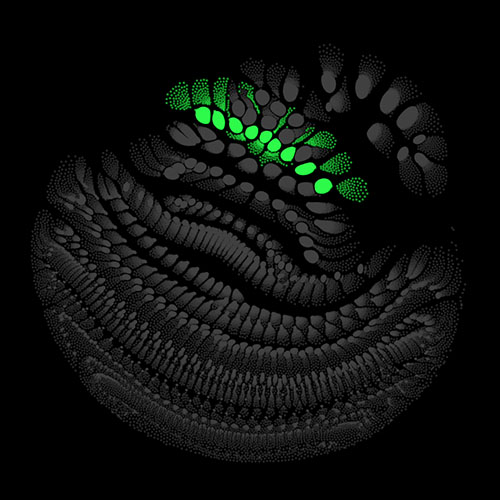
Visualization
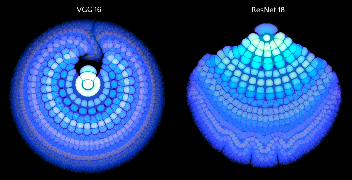
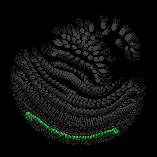
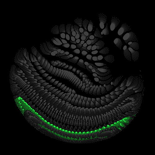
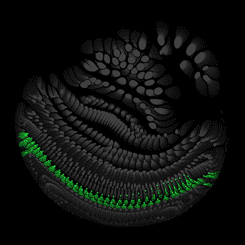
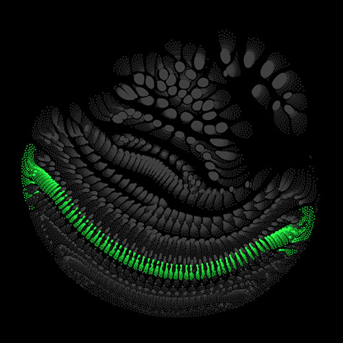
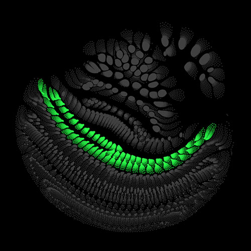
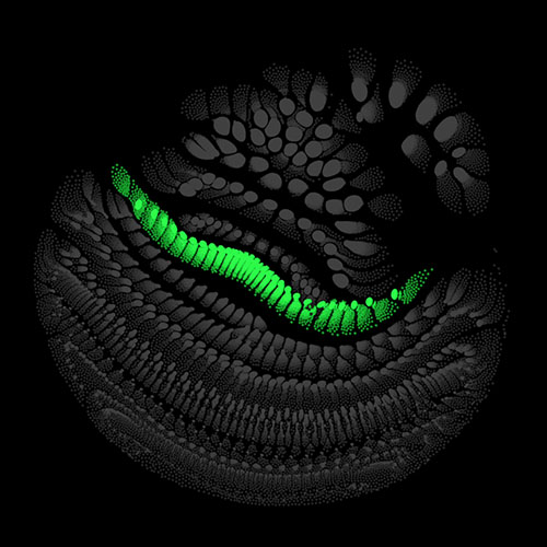
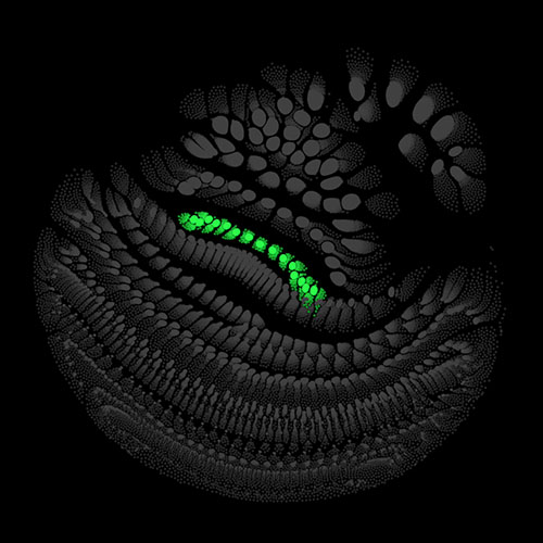
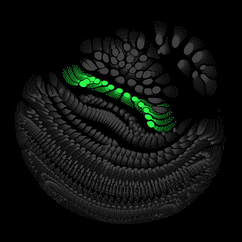
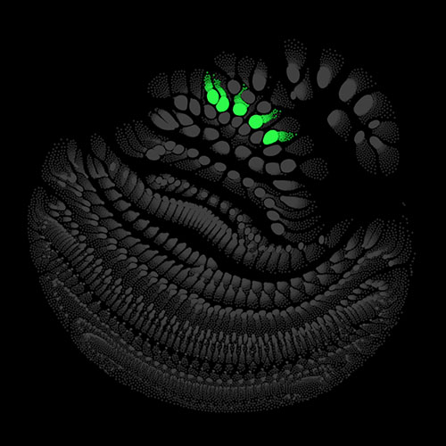
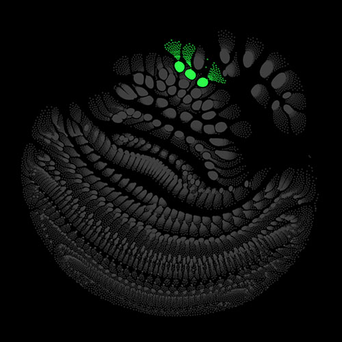
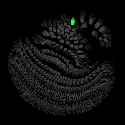
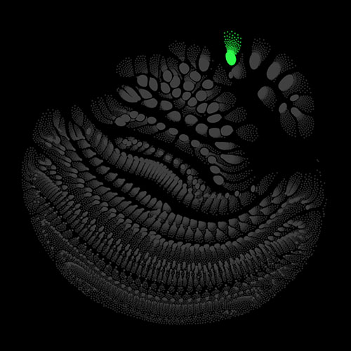
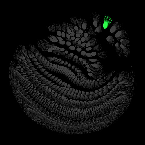
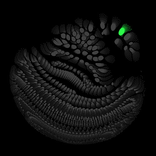
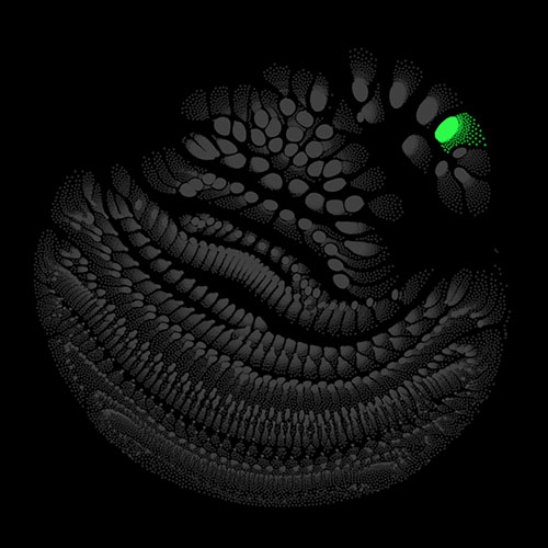
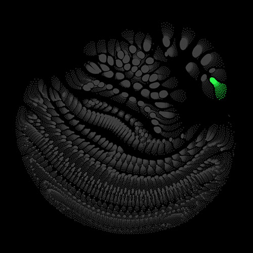
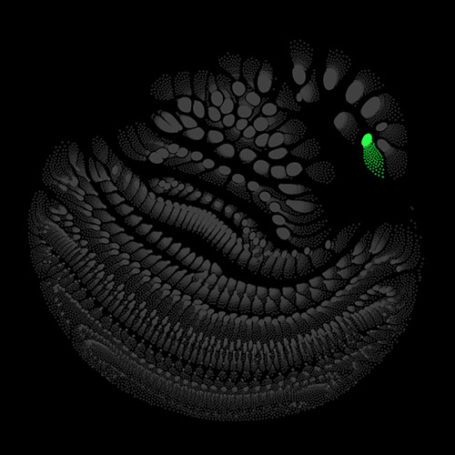
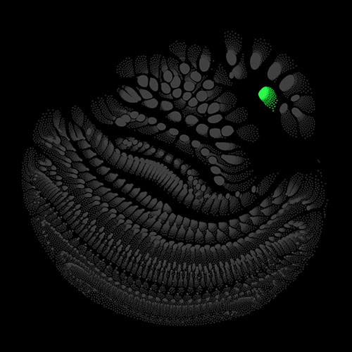
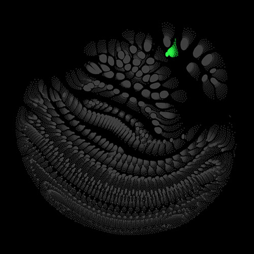
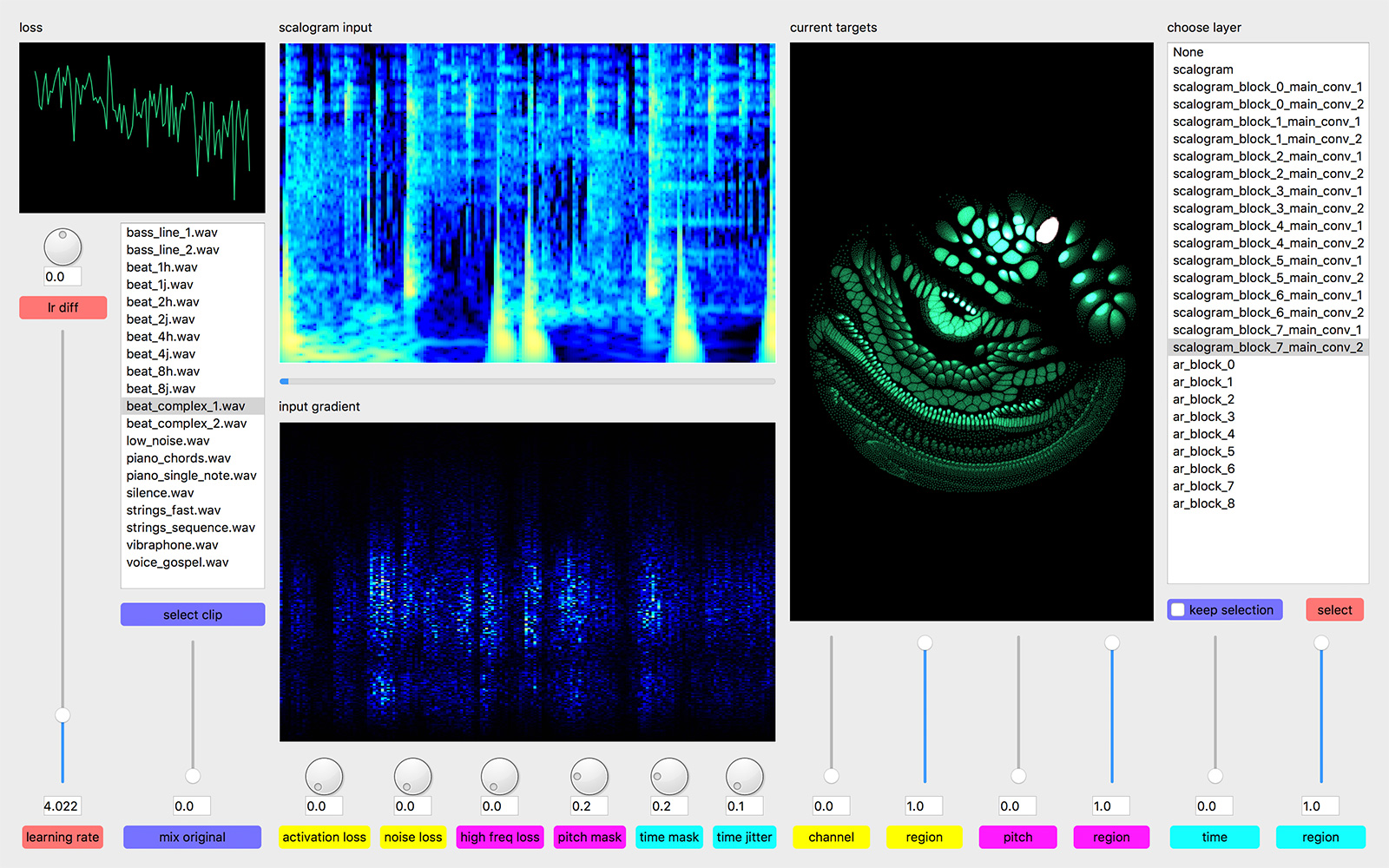
To illustrate what is going on inside the model at each moment, we visualize the activation of the artificial neurons (i.e. the outputs of the nonlinearities). The place of each neuron in our network can be described by four coordinates: layer, frequency, time, and channel. We treat the time dimension different from the other dimensions and exclude it for now. The neurons can be seen as the vertices of a graph. They are connected in different patterns by edges, depending on the type of layer (e.g. fully connected or convolutional) the neurons belong to. There exist methods to lay out graphs into suitable shapes. For our purposes, the force layout technique is the best fit. Here the graph is modelled as a physical system with different forces acting on the vertices. The system, starting from random initial conditions, can be simulated using numerical methods, e.g. Verlet integration.
In our setting, there are three types of forces acting on each vertex. The first force pulls together vertices that are directly connected. The strength is proportional to the distance between vertices and can be scaled with the weight of the connecting edge. Formally, the attractive force $\mathbf{a}$, caused by vertex $j$ and acting on vertex $i$, with their respective positions $\mathbf{p}$, and connected by an edge with weight $w_{ij}$, is:
\[\mathbf{a}_{ij} = w_{ij} \, (\mathbf{p}_j - \mathbf{p}_i)\]If there vertices $i$ and $j$ connected, $w_{ij}$ is $0$. In practice, the attractive forces are calculated only for connected vertices.
The second force works as if each vertex had a certain electric charge, which would make vertices repel each other. The force $\mathbf{r}$ caused by vertex $j$ and acting on vertex $i$, and charges $q$, is:
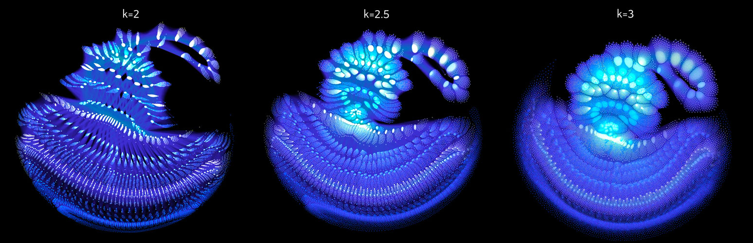
\[\mathbf{r}_{ij} = q_i q_j \, \frac{\mathbf{p}_i - \mathbf{p}_j}{\|\mathbf{p}_i - \mathbf{p}_j\|^{k+1}}\]For a physically accurate simulation of an electrostatic force, the exponent $k$ would have to be 2. But seen as an adjustable parameter, it gives us some control over the appearance of the layout: it controls which of the forces, repulsive and attractive, dominates at a given distance between vertices. For high values of $k$, the repulsive force is strong over short and weak over long distances. This leads to the vertices being more evenly spread out. On the other hand, low values of $k$ result in dense clusters of vertices.
The optional centering force, scaled by a global factor $l$, pushes vertices towards the origin:
\[\mathbf{c}_{i} = -l \, \mathbf{p}_i\]With that, the combined force $\mathbf{f}$ acting on vertex $i$, can be defined as:
\[\mathbf{f}_{i} = \mathbf{c}_{i} + \sum_{j \neq i} \mathbf{r}_{ij} + \mathbf{a}_{ij}\]Since the number of individual forces that have to be calculated scales quadratically with the number of vertices, for large networks it is necessary to approximate the forces $\mathbf{r}_{ij}$ in a computationally efficient way using the Barnes-Hut-tree method.
To avoid local energy minima, it is helpful to start the simulation with a low-resolution graph and increasing the resolution in steps until the full graph reached. For our neural networks, the construction of lower resolution levels can be done by iteratively consolidating vertices that are neighbouring in the channel or the frequency dimension. The expansion is done in the inverse order. Also, it can be helpful to slowly increase the centering force factor with each new resolution level.
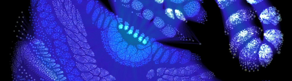
There are many possibilities on how to determine the weights of the edges and the charges of the vertices. I chose to use uniform weights for the edges and use the variance of the activation of each neuron across the validation set as its charge. For each point in the time dimension, which we excluded above, we get different charge values for the vertices, which means also results in a slightly different layout. Calculating several of these snapshot layouts allows us to construct an animated version of the network. Once the layout is worked out the current state of the net can be depicted by lighting up strongly activated neurons and letting others stay dark.
The code for the GPU accelerated layout calculation (implemented in PyTorch) and the OpenGL-based visualization is available here.
Input Optimization
Today’s neural networks usually are completely differentiable. This means we can generate inputs for a trained model that maximize the activations of certain neurons in the network using iterative gradient-based optimization. These inputs can then be directly experienced by humans and show which particular stimuli the selected neurons respond to. In our case, this procedure sonifies the features activating the selected neurons.
Neural nets, especially if they did not receive adversarial training, are susceptible to small changes in the input. These can lead to local optima that are not perceptible by humans but still have the required properties. To prevent this, several types of regularization are applied: temporal shifting of the input, small pitch changes, masking of random regions in the scaleogram, noisy gradients and de-noising of the input. All these methods make the input optimization more difficult in certain ways and thus enforce more robust and distinct results.
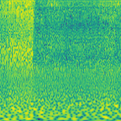
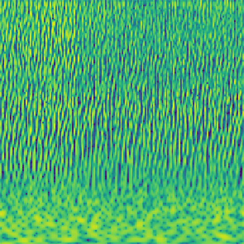
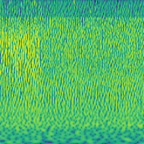
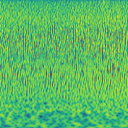
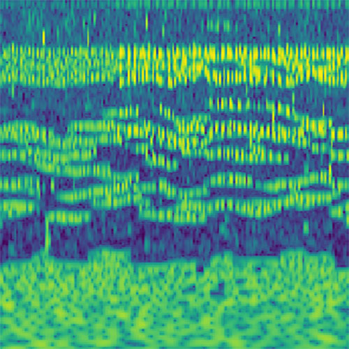
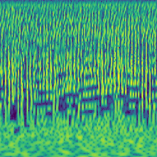
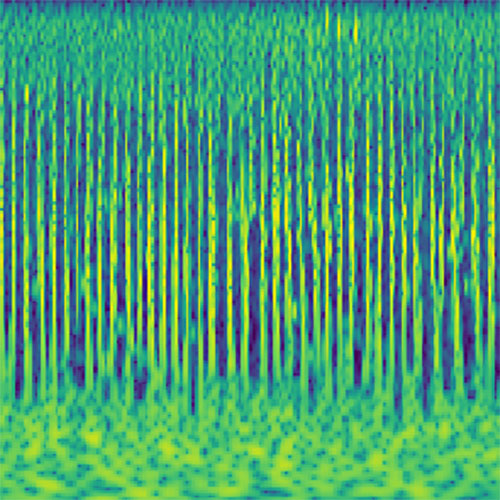
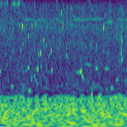
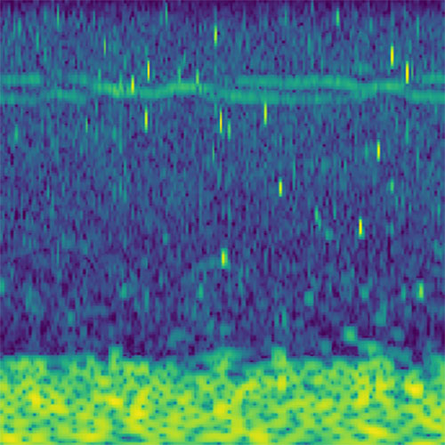
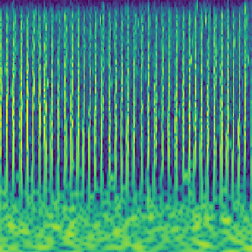
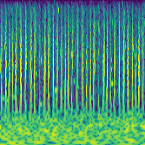
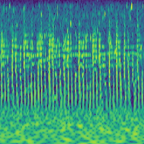
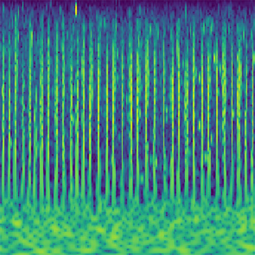
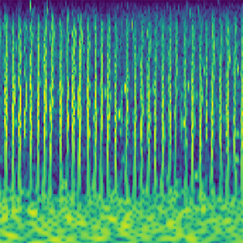
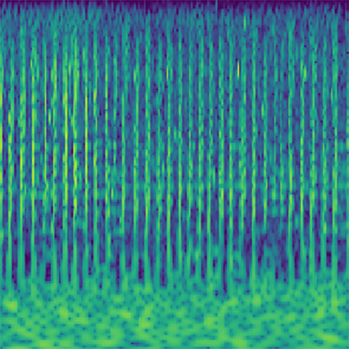
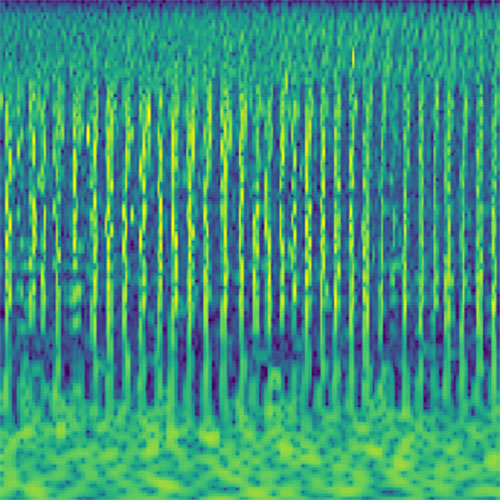
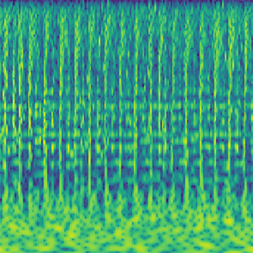

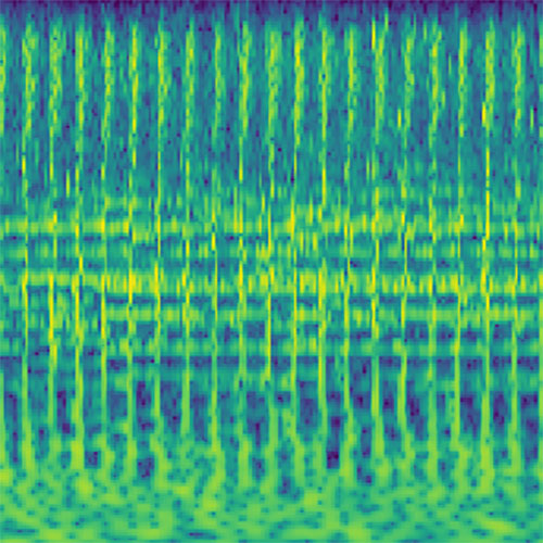
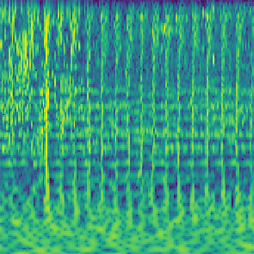
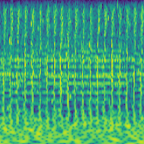
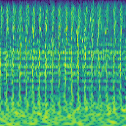
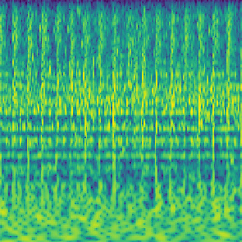
Audio clips that maximize the activation of the selected layer. The right pictures show the scaleogram representations.
Live Performance
Like the inputs, the generated audio clips have a duration of about four seconds. With that, they lend themselves for a loop-based live performance. One loop then corresponds for example to two 4/4 measures at 120 bpm. The optimization procedure described above constantly generates new audio clips. As soon as one clip has finished playing, the latest newly calculated clip is started. An acoustic morphing arises as a result that is also reflected in the visualization (each pattern of activations yields its own distinct sounds). As origin for the optimization silence and noise can be used as well as a pre-built clip that for example dictates a certain rhythm.
A quick journey through some selected activations, starting from silence.
All aspects of the procedure can be adjusted in real-time. For intuitive control, I developed a GUI and made the most important parameters controllable by a MIDI controller. The setup described here is very flexible, other networks trained on different data or with different architectures can easily be employed.
Leave a Comment